Transformer Attention Internals
A differentiable, content-addressable soft lookup: every token computes a query, matches it against every token's key, and pulls a softmax-weighted blend of their values — in one parallel hop. The mechanism behind every modern foundation model (Vaswani et al., 2017).
What · How · Why
What it is
Attention lets every token in a sequence directly look at every other token and pull in a weighted blend of their information, where the weights are computed dynamically from the content itself. Self-attention is the core operation; the Transformer is the architecture built by stacking it. It replaced recurrence and convolution as the default for sequence modeling.
How it works
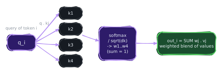
Each token's embedding is projected into a Query ("what I'm looking for"), a Key ("what I offer"), and a Value ("what I hand over"). A token's query is dotted against all keys, scaled by \(1/\sqrt{d_k}\), softmaxed into weights summing to 1, and used to take a weighted sum of the values. Multi-head runs several of these in parallel; positional encodings inject order.
Why it matters
It solves the two fatal flaws of RNNs at once: long-range dependencies (any token reaches any other in a constant-length path, not hundreds of decaying steps) and parallelism (it's matrix multiplies, so the whole sequence trains at once on GPUs). That combination — not a single benchmark win — is why it took over.
Round 1 — Mental Model
Picture a meeting room where everyone speaks at once but you hold a directional microphone. Each person holds up a sign saying what they care about (their query) and wears a badge saying what they know about (their key). You aim your mic toward the people whose badges best match your sign, and the softmax is the gain knob — it decides how much of each person's voice (their value) makes it into your notes. The matching is content-based and recomputed at every layer, so who you listen to changes as understanding deepens.
Contrast the RNN: a game of telephone down a line. By the time a message from the first speaker reaches you it has passed through hundreds of mouths and degraded. Attention lets you talk to the original speaker directly — one hop, no decay.
Round 2 — Internal Mechanics & Mathematical Model
Formal definition
Given input \(X \in \mathbb{R}^{n \times d}\) (n tokens, model dim d), project to queries, keys, values with learned matrices \(W_Q, W_K \in \mathbb{R}^{d \times d_k}\), \(W_V \in \mathbb{R}^{d \times d_v}\):
\[ Q = XW_Q,\quad K = XW_K,\quad V = XW_V \]Key equation (scaled dot-product attention)
\[ \operatorname{Attention}(Q,K,V) = \operatorname{softmax}\!\left(\frac{QK^{\top}}{\sqrt{d_k}}\right) V \]\(QK^{\top}\in\mathbb{R}^{n\times n}\) is the matrix of all pairwise query–key dot products; row \(i\) softmaxed gives token \(i\)'s attention distribution over all tokens; multiplying by \(V\) takes the corresponding weighted sums.
Derivation sketch — why \(1/\sqrt{d_k}\)?
Assume the entries of \(q\) and \(k\) are independent, zero-mean, unit-variance. A single dot product is \(q\cdot k=\sum_{m=1}^{d_k} q_m k_m\). Each term has mean 0 and variance 1, and they're independent, so
\[ \operatorname{Var}(q\cdot k)=\sum_{m=1}^{d_k}\operatorname{Var}(q_m k_m)=d_k \]So the logits have standard deviation \(\sqrt{d_k}\) and grow with dimension. Large logits push softmax into a saturated, near-one-hot regime where its Jacobian \(\approx 0\) — gradients vanish. Dividing by \(\sqrt{d_k}\) rescales the variance back to 1, keeping softmax in its responsive region. This is the entire reason the scale factor exists.
Multi-head attention
\[ \operatorname{MHA}(X)=\operatorname{Concat}(\text{head}_1,\dots,\text{head}_h)\,W_O,\quad \text{head}_i=\operatorname{Attention}(XW_Q^i,XW_K^i,XW_V^i) \]Each head uses \(d_k=d/h\), so total compute is roughly constant in \(h\). Heads specialize — empirically some track syntactic adjacency, some long-range coreference, some positional offsets.
Complexity analysis (the central fact)
Time: \(QK^{\top}\) is \(n\times d_k\) times \(d_k\times n\) = \(O(n^2 d_k)\); the \(\cdot V\) is again \(O(n^2 d_v)\). So self-attention is \(O(n^2 d)\) time and \(O(n^2)\) memory — quadratic in sequence length. Why quadratic: every token attends to every token, so the score matrix has \(n^2\) entries by construction. This single fact drives almost every systems concern downstream (long-context cost, KV cache, FlashAttention, linear-attention variants).
Contrast: an RNN is \(O(n d^2)\) time — linear in \(n\) — but with a sequential dependency of depth \(n\) (path length \(O(n)\)), so it can't parallelize over the time axis. Attention trades linear-compute-but-sequential for quadratic-compute-but-fully-parallel and path length \(O(1)\). On GPUs that trade is overwhelmingly worth it up to long contexts.
Invariants
(1) Rows of the softmax sum to 1 — each output is a convex combination of values, so it lives in their convex hull (bounded, no blow-up). (2) Permutation equivariance — without positional encoding, permuting input tokens permutes outputs identically; attention has no intrinsic order, which is exactly why positional information must be added. (3) Gradient flows in one hop between any two positions — the property that defeats vanishing gradients over distance.
Limiting cases
As the temperature → ∞ (logits → 0, e.g. all keys identical), softmax → uniform and attention returns the plain mean of values — it becomes order-agnostic average pooling. As temperature → 0 (one logit dominates), softmax → one-hot and attention becomes a hard lookup (argmax retrieval). With \(n=1\), attention is the identity on that token's value. As \(n\to\infty\), the \(O(n^2)\) memory wall is what forces approximate/linear attention.
Round 3 — Where It Breaks & Expert Debates
The quadratic wall. \(O(n^2)\) memory caps practical context length and dominates long-document / long-context cost. A decade of work attacks it: sparse attention (Longformer, BigBird), low-rank/linear attention (Linformer, Performer), and — the one that actually won in practice — FlashAttention, which doesn't change the math but tiles the computation to keep the \(n\times n\) matrix out of HBM, making it IO-aware. Debate persists over whether sub-quadratic approximations ever match full attention's quality, or whether the right move is exact-but-IO-efficient.
Is attention even necessary? State-space models (S4, Mamba, 2023–24) recover near-Transformer quality with linear-time recurrence, reopening the question of whether the quadratic all-to-all interaction is fundamental or just convenient. Strong opinions on both sides; unsettled as of 2026.
Attention weights ≠ explanation. A well-known debate ("Attention is not Explanation," Jain & Wallace 2019, vs "Attention is not not Explanation," Wiegreffe & Pinter 2019): high attention weight on a token does not reliably mean that token caused the prediction. Treating attention maps as interpretability is contested.
Positional encoding is unsolved-ish. The original sinusoidal scheme generalizes poorly to lengths beyond training. RoPE and ALiBi improve extrapolation but length generalization remains an active failure mode — models trained at 4k context degrade well before truly arbitrary lengths.
Round 4 — AI × Networks Connection
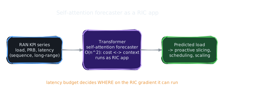
Attention is the model class that makes network traffic prediction tractable as a sequence problem: cell-level KPI and load time-series are exactly "sequences with long-range, multi-scale dependencies" (daily + weekly seasonality, sudden bursts), which is where attention beats RNNs. A Transformer forecasting head running as an O-RAN rApp/xApp is one of the cleanest deployable intersection artifacts — and its \(O(n^2)\) cost is precisely why where it runs on the RIC latency gradient matters.
The second non-obvious link is serving economics: the quadratic-memory fact from Round 2 is the same constraint that governs LLM-on-K8s serving (KV cache size, batch vs latency tradeoffs). The systems intuition transfers directly between "serving a Transformer" and "placing an inference xApp under a latency budget" — both are memory-bound, batch-sensitive inference-at-the-edge problems.
Cross-links
Networks · O-RAN architecture → the substrate where a Transformer forecaster is deployed as a RIC app, under the latency gradient.
Papers · Attention Is All You Need (Vaswani 2017) → the source paper for this node's mechanism.
Papers · Back-propagation (1986) → the credit-assignment that trains the learned Q/K/V projections.
Pending intersection / AI nodes this unblocks: KV cache mechanics & inference memory layout, Transformer models for traffic prediction, LLM serving on K8s, LLM for network config generation.
Open questions this raises
- For RAN traffic prediction, does full \(O(n^2)\) attention actually beat a linear-time state-space model (Mamba), or is the all-to-all interaction wasted on KPI series with mostly local + periodic structure?
- Given the RIC latency floor (~10 ms near-RT), what context length \(n\) and head count \(h\) are even admissible for an inference xApp? Where's the Pareto frontier of accuracy vs serving latency?
- Should KV cache mechanics and positional-encoding schemes (RoPE/ALiBi) be separate KB nodes or sub-sections here — i.e. how fine-grained should node granularity be?
- Does the "lost in the middle" dilution failure manifest in long KPI windows, and does it bias which historical events the forecaster attends to?