ImageNet Classification with Deep Convolutional Neural Networks

papers Krizhevsky, Sutskever & Hinton · 2012 Round 4 ✓ math ✓ visual ✓

"AlexNet" — the result that ignited the deep-learning era. By training a deep CNN on GPUs with ReLU and dropout, it cut ImageNet top-5 error from 26.2% to 15.3%, ending the hand-engineered-feature paradigm in computer vision overnight.

What · How · Why

What it is

"AlexNet" — the deep convolutional network that won the 2012 ImageNet competition by a stunning margin and ended the era of hand-engineered image features. It is the empirical result that converted the field to deep learning almost overnight.

How it works

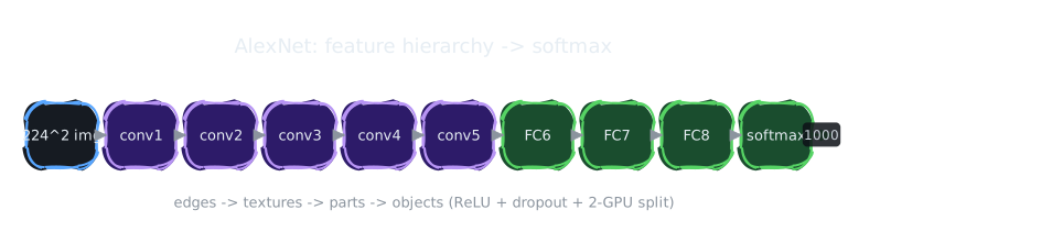
It stacks learned convolutional filters that build a hierarchy — early layers detect edges and colors, middle layers textures and parts, late layers whole objects — all trained end-to-end by backpropagation. The breakthrough was making this work deep: ReLU activations (which don't saturate, so gradients survive), dropout (randomly disabling units to prevent a 60-million-parameter net from memorizing), data augmentation, and splitting training across two GPUs to fit in memory.

Why it matters

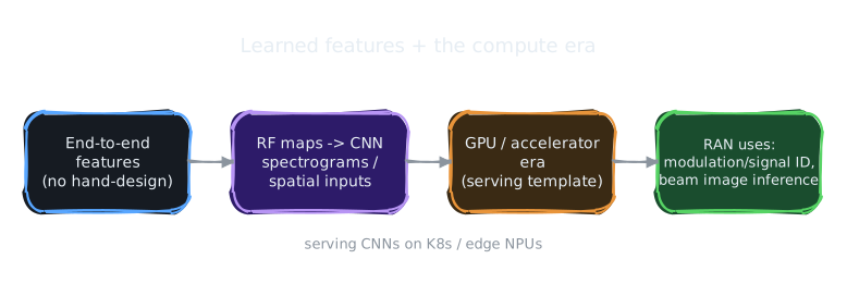
It ignited the deep-learning era and the GPU-for-AI economy, and established the recipe — deep network + big data + accelerators + regularization — that the Transformer would later scale. It also set the deployment template you work in: serving deep models on GPUs/edge NPUs, now used for RF/PHY tasks like modulation and signal classification from spectrograms.

Round 1 — Core Claim & Mental Model

The problem it solves

Until 2012, image recognition meant hand-crafted features (SIFT, HOG) + a shallow classifier. The claim: a deep CNN, given enough data (ImageNet, 1.2M images) and compute (GPUs), learns better features end-to-end than humans can design — if you solve the practical training obstacles.

Mental model

A hierarchy of learned filters. Early layers detect edges and color blobs; middle layers compose them into textures and parts; late layers assemble parts into objects. Convolution = the same small filter slid everywhere (translation-equivariance + weight sharing), so the net learns "edge detector" once and reuses it across the image.

Why now (2012) and not 1989? Three things aligned: big labeled data (ImageNet), parallel compute (CUDA on GTX 580s), and training tricks (ReLU, dropout) that tamed backprop at depth. The algorithm was old; the ecosystem finally caught up.

Round 2 — Mathematical Model

Convolution layer

\[ y_{i,j,k} = \sigma\!\Big( b_k + \sum_{c}\sum_{u,v} W_{u,v,c,k}\,x_{\,i+u,\,j+v,\,c} \Big) \]

Filter \(W\) of size \(f\times f\times C\) produces feature map \(k\); shared across all positions \((i,j)\).

The key ingredients

ReLU: \(\sigma(z)=\max(0,z)\). Non-saturating, so gradients don't vanish — they report ~6× faster convergence than tanh. Dropout: randomly zero hidden units with prob 0.5 at train time, \(\approx\) averaging an exponential ensemble — the main regularizer for the 60M-parameter net. Local response normalization and overlapping max-pooling add competition and small translation invariance.

Architecture & size

5 convolutional + 3 fully-connected layers, ~60M parameters and ~650K neurons, ending in a 1000-way softmax. Trained split across two GPUs (3GB each) — an early model-parallelism necessity, not a choice.

Complexity

Conv cost per layer: \(O(H\,W\,C_{\text{in}}\,C_{\text{out}}\,f^2)\) — dominated by spatial size × channels × kernel area. Weight sharing makes parameter count tiny relative to a fully-connected equivalent (a key reason it fit in memory), but FLOPs stay high — the GPU was essential. Inference is feed-forward \(O(\text{FLOPs})\).

Invariants & limiting cases

Convolution is translation-equivariant by construction (shift input ⇒ shift feature map). Limiting cases: \(1\times1\) filters reduce to per-pixel MLPs (channel mixing only); remove pooling and the receptive field grows only linearly with depth; remove dropout and the 60M-param net overfits 1.2M images badly — the authors report dropout was essential.

How It Works & Visual Diagrams

AlexNet pipeline — Architecture: 5 conv + 3 FC layers. Spatial size shrinks while channel depth/abstraction grows — the canonical CNN funnel.

AlexNet and networks — Intersection diagram: AlexNet established learned features + GPU serving — the deployment template (CNNs on K8s/edge NPUs) now used for RF signal/modulation classification and spatial RAN inference.

Mathematical Proofs

AlexNet has no single theorem; its power comes from three structural choices, each of which admits a clean formal statement: convolution is translation-equivariant (and parameter-thrifty), ReLU removes the gradient-killing factor of backprop, and dropout is an expectation over an exponential ensemble.

Proposition 1 — Translation equivariance of convolution Let \(T_\tau\) shift an input by \(\tau\), \((T_\tau x)[p]=x[p-\tau]\), and let \(C_W\) be cross-correlation with kernel \(W\). Then \[ C_W(T_\tau x)=T_\tau\big(C_W(x)\big): \] a shifted input produces a shifted feature map. This is the inductive bias that lets one learned filter detect a pattern anywhere.

Proof. By definition \(C_W(x)[p]=\sum_{u}W[u]\,x[p+u]\). Substitute the shifted input: \[ C_W(T_\tau x)[p]=\sum_u W[u]\,(T_\tau x)[p+u]=\sum_u W[u]\,x[p+u-\tau]=C_W(x)[p-\tau]=T_\tau\big(C_W(x)\big)[p]. \] Equality for all \(p\) is the claim. (Note convolution is equivariant, not invariant; pooling adds approximate invariance by discarding the shifted index.) ∎

Proposition 2 — Weight sharing & cost A conv layer with \(C_\text{in}\) input channels, \(C_\text{out}\) filters of size \(f\times f\), output \(H\times W\), uses \(f^2C_\text{in}C_\text{out}\) weights and \(2f^2C_\text{in}C_\text{out}HW\) FLOPs — independent of spatial position. A fully-connected layer over the same map would need \((HWC_\text{in})(HWC_\text{out})\) weights, larger by a factor \(\sim H^2W^2/f^2\).

Proof. Each of the \(C_\text{out}\) filters has \(f^2C_\text{in}\) weights, reused at every output location (sharing), giving \(f^2C_\text{in}C_\text{out}\) parameters; each output element costs one multiply-add (2 FLOPs) per weight over \(HW\) locations. The dense alternative connects every input unit \(HWC_\text{in}\) to every output unit \(HWC_\text{out}\). The ratio \(\dfrac{H^2W^2C_\text{in}C_\text{out}}{f^2C_\text{in}C_\text{out}}=\dfrac{H^2W^2}{f^2}\) is the parameter saving — millions-to-thousands for real maps, the reason CNNs train on limited data. ∎

Proposition 3 — Dropout = expectation over a sub-network ensemble With independent keep-probability \(p\) masks \(m_i\sim\mathrm{Bernoulli}(p)\), a unit's expected pre-activation equals the deterministic test-time unit with weights scaled by \(p\): \[ \mathbb E_m\Big[\textstyle\sum_i w_i\,(m_i x_i)\Big]=p\sum_i w_i x_i. \]

Proof. By linearity of expectation and \(\mathbb E[m_i]=p\): \(\mathbb E_m[\sum_i w_i m_i x_i]=\sum_i w_i x_i\,\mathbb E[m_i]=p\sum_i w_i x_i\). Hence the “weight-scaling rule” (multiply weights by \(p\) at inference) reproduces, for a single linear layer, the mean over the \(2^{n}\) possible drop patterns — an exponentially large ensemble averaged at the cost of one network. For deep nonlinear nets this is an approximation (geometric-mean ensemble), which is why dropout regularizes rather than computes an exact average. ∎

Proposition 4 — ReLU preserves the gradient For \(\sigma(z)=\max(0,z)\), \(\sigma'(z)=1\) on active units (\(z>0\)), versus \(\sigma'\le\tfrac14\) for the logistic sigmoid. The per-layer Jacobian factor is therefore \(1\) on the active path, removing the exponential decay of backprop.

Proof. Differentiate piecewise: for \(z>0\), \(\tfrac{d}{dz}z=1\); for \(z<0\), \(\tfrac{d}{dz}0=0\). In the depth-\(L\) gradient product \(\prod_l \mathrm{diag}(\sigma'(z^{(l)}))(W^{(l)})^{\top}\), sigmoid contributes factors \(\le\tfrac14\) (so \(\le 4^{-(L-1)}\) shrinkage before weights act), while ReLU contributes exactly \(1\) on active units — only the weight spectra then govern signal scale. The cost is the “dying ReLU” at \(z<0\) (zero gradient), motivating Leaky/ELU variants. ∎

Cross-links: equivariance and weight-sharing make CNNs the deployment template for RF signal/modulation classification and spatial RAN inference on edge NPUs; the ReLU result is the practical unlock of backpropagation, and the same residual/normalization toolkit reappears in the Transformer.

Round 3 — Limitations & Community Response

Data- and compute-hungry; weak priors beyond translation. AlexNet needed 1.2M labels and GPU weeks. CNNs encode translation but not rotation/scale invariance, and are notoriously brittle to adversarial perturbations and distribution shift — vulnerabilities discovered shortly after (Szegedy 2013).

Rapid supersession. The architecture was quickly improved: VGG (deeper, smaller filters), GoogLeNet/Inception, and especially ResNet (2015), whose residual connections enabled 100+ layers and pushed ImageNet error below human level. AlexNet is historically pivotal but architecturally obsolete.

Reception. The single most important empirical result in modern AI's takeoff — it converted the field to deep learning and triggered the GPU-for-AI economy. Critiques target generalization and robustness, not the headline result, which has been reproduced exhaustively.

Round 4 — AI × Networks Connection

AI lineage. AlexNet is backprop (1986) finally working at scale, and the proof-of-concept that made the Transformer's scaling bet credible five years later. It established the modern recipe: deep net + big data + accelerators + regularization. It connects the early-NN papers to the foundation-model era.

Networks angle. CNNs are now standard for RF/PHY tasks — modulation classification, signal/interference identification, and treating spectrograms or spatial beam patterns as images. Just as important, AlexNet set the deployment template you work in: serving deep models on GPUs/edge NPUs, with the latency/throughput tradeoffs that dominate inference-at-the-edge for RAN.

→ Backprop 1986 (the optimizer) → Attention 2017 (next architecture) → GPT-3 2020 (scaling continued)

Verify — Credibility Check

Headline numbers (confirmed): ILSVRC-2012 top-5 error 15.3% vs the next-best 26.2% — a ~10.9-point gap, unprecedented in the competition's history; ~60M parameters, 650K neurons, 5 conv + 3 FC layers, trained on two GTX 580 GPUs. Plausibility is unimpeachable: the result was won live in a public benchmark, code/weights were released, and it has been reimplemented thousands of times. The single experiment that validated it was the ImageNet leaderboard itself; the field's immediate pivot to deep learning is the strongest possible external confirmation.

Open questions this raises:

For RF/PHY tasks, do convolutional priors (translation equivariance) actually match the symmetries of spectrogram/IQ data, or do attention/SSM models fit RAN signals better?
What is the right accelerator/quantization point to serve a CNN classifier inside a RAN latency budget — and how does that compare to the AlexNet-era GPU template?
Given CNN adversarial brittleness, how robust must a deployed RF classifier be to deliberate interference, and does that change the architecture choice?